Fd3d_xy, is the distribution version of the 3D finite difference program to model dynamic rupture developped at UCSB and ENS by K.B. Olsen, R. Madariaga and R. Archuleta.
Contents
1. Methodology
2. Distribution
3. Running the program
4. Output and plotting
5. References
PLEASE NOTE: these are minimal notes permitting the use of this program. They are not conceived and cannot be used as a tutorial on finite differences.
fd3d_xy is a finite difference program developped in order to model dynamic seismic rupture propagation along a planar fault situated on the xy plane of an elastic medium. The Finite difference volume and the position of the fault are shown in Figure 1
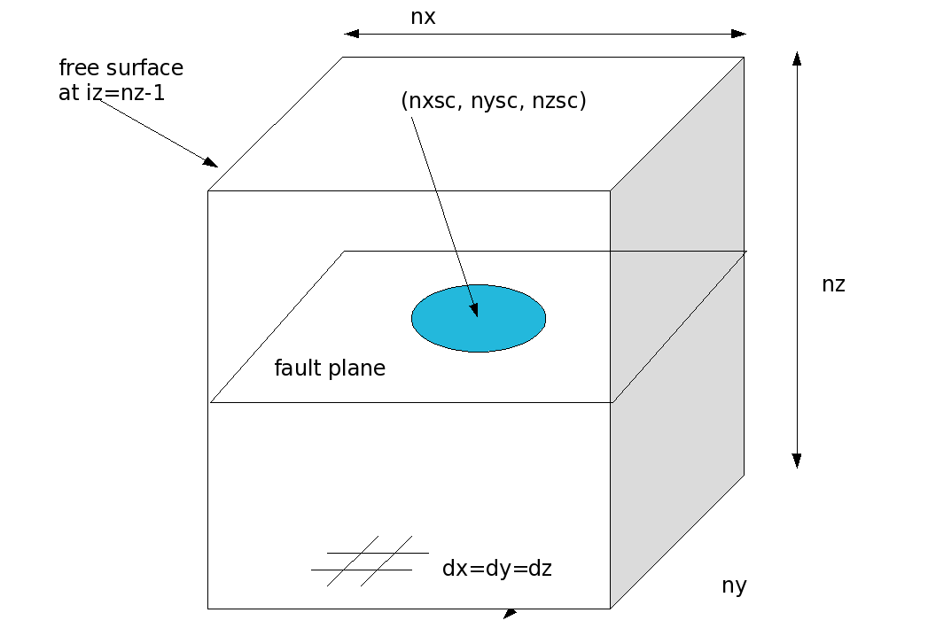
Figure1. The Finite difference volume.
The program computes wave propagation produced by the rupture on a grid NX by NY by NZ points. The curve is surrounded by absorbing boundary conditions of the Clayton-Engquist type except at the top of the cube on the NZ line which is treated as a free surface. This can be easily changed if a cube fully surrounded by absorbing B.C. is wished. A version with PML boundary conditions is also available, but it can not be distributed for the moment. PML do not change the results very much but are very delicate to implement.
1. METHODOLOGY
The present version is based on the theory presented by Madariaga, Olsen and Archuleta, Modeling dynamic rupture in a 3D earthquake fault model, Bull. Seismol. Soc. Am., 88, 1182-1197, 1998.
The finite difference method used by this program is a 4th order staggered grid velocity stress method based on earlier work by Madariaga (1976), Virieux (1983), Levander (1988) and Olsen (1992).
1.2 Crack Boundary Conditions (and my philosophy about them)
There has been an abundant literature on boundary conditions for simulating earthquake ruptures. Two approaches are possible:
(1) Split nodes where the fault is treated as an internal boundary of the elastic medium. This method can be used together with symmetry conditions in order to solve the problem on half the volume (See Madariaga, 1976, Andrews, 1974). In finite differences this approach produces strong oscillations because it looses precision near the fault. It is necessary to use artificial damping in order to get good stable solutions.
(2) Thick or thin boundary conditions, where faulting is simulated by a continuum approach where the the fault is treated like an inclusion in order that stress and slip satisfy the friction law. The crack boundary conditions are either thick or thin fault boundaries depending on the thickness of the layer of transformational strain (seismic moment) that is used. These boundary conditions preserve symmetry about the fault plane and they do not need any artificial damping.
The program fd3d_xy uses thin boundary conditions without any artificial damping. Unfortunately, in the BSSA paper by Madariaga et al cited above we only described the thick boundary conditions. Thin boundary conditions are just a small change from those. All it takes is to delete two lines from the code. Many authors claim that thin faults are more accurate than thick ones because they give better results for the SCEC model test. Actually when properly scaled the results are fully equivalent, but thin BCs are more efficient.
1.3 Stability and dispersion
Numerical stability and dispersion of fd3d_xy is controlled by the largest value of the P wave velocity, Vpmax through the so-called CFL non-dimensional number
H=Vpmax*dt/dx
For stable propagation in the bulk, with minimum dispersion H<=0.5. Yet the boundary conditions become unstable for such value of H. Our practice shows that an optimal value is H<=0.25.
2. DISTRIBUTION
The distribution tar-ball contains three directories
Directory <src_xy>
Contains the fd3d_xy program and its subroutines as well as some auxiliary programs that are useful in generating initial stresses and rupture resistance. Makefile compiles all the programs using the standard GNU gfortran compiler. If you are using a different compiler please redefine the $F77 variable in the makefile to suit your compiler. I have commented out the compiler line I use for the intel compiler. INTEL compiler produces a faster code but is not free.
Directory <bin>
Contains the compiled programs using the most recent version of gfortran (4.1.2)
Directory <circular_crack>
Contains an example that runs the fd3d_xy program with a set of initial conditions generated by the mkdata.run program. This is a rather straightforward method to generate a simple initial stress and yield stress distribution to run the fd3d_xy program. We call this example circular because rupture stops at a strong barrier of circular shape. Other shapes can be easily introduced using the options to the mkdata program. Please read the mkdata.f file in the src_xy directory for minimum instructions.
The circular crack example uses a cube of size 160^3. You can run on smaller cubes but the resolution will be too poor for any practical use. With thin boundary conditions our program requires at least 10 grid points per wavelength and at the very least 7 points on the slip weakening (or process zone). Some authors claim that FDs can solve the friction law even with fewer sampling points on the slip weakening zone (Dalguer and Day, JGR, paper B02302, 2007). I do not support such claims for the fd3d_xy code.
The circular example runs in less than 1 hour in any modern linux work station.
PREPARING STRESS DATA
The example included circular has been tested on several computers and compilers. It should work ;)
The script mkdata.run uses the mkdata program to produce a peak.ini file that defines a rupture zone low peak stress of radius 80 grid points centered on the central point (80,80) of the fault plane. Peak (yield) stress is 8 MPa inside the circle and 160 MPa outside. This produces an unbreakable barrier around the circular fault. The second line on the mkdata.run script defines a weak circular zone of radius 15 grid points where strength is reduced by 3.5 Mpa to only 4.5 MPa. This is the triggering asperity.
File stressx.ini defines an initial stress field on the fault that is equal to 5 MPa everywhere.
Test yourself other values, but remember that the numbers above where chosen so that rupture starts and then accelerates up to about 80% of the shear wave speed. So change them moderately !
Note that it may be probably simpler to write your own version of mkdata.
The MODEL.DAT File
The fd3d_xy can propagate waves from an arbitrarily stratified velocity model, but the crack boundary conditions using the thin fault methodology only work if the fault is inside a homogeneous layer. Thus, the velocity density model has to be stratified along the z direction because the fault itself, defined by its central point nxsc,nysc,nzsc, has to be on a homogeneous layer. fd3d_xy can not compute bi material faults.
The model.dat file provided in the circular crack model is easy to generate with a few lines of FORTRAN if you want to change it.
The INPUT.DAT File
This is the file that controls the program. This file contains grid sizes, defines the points where you want to print output data, etc.
File input.dat should be self-explanatory, I hope.
At the bottom of the input.dat file you can specify up to 100 sites where you can get velocity and displacement seismograms. These sites are specified by their 3 coordinates in space. Please remember that the fault is on the nzsc plane of the grid and the free surface at iz=nz-1. Currently the seismograms are printed with fixed format to file unit 28. You may want to change this in subroutine wrss3d.
There are several lines identified by
c
c write isolated seismograms
c
if(nholes.gt.0)then
write(28,'(12g14.5)')time,(u2(nbhx(j),nbhy(j),nbhz(j)),
$ j=1,nholes)
Now you are ready to run the bash-shell script fd3d_xy.run. After less than 1 hour you should get the results
The output of the program is written in the sub directory <results>.
The program produces a series of snapshots as follows:
sliprate.res is the sliprate as a function of position on the fault plane. In order to save space point on the fault are decimated according to the variables NBGX,NEDX, NSKPX and NBGY,NEDY,NSKPY defined in the input.dat file
slip.res contains slip distribution on the fault decimated in the same way as sliprate.res
ssx3d.res this is the x component of stress sigma_{xz} on the fault plane decimated in the same way as sliprate.
ssy3d.res is the sigma_{yz} component of stress on the fault
ssz3d sigma_{zz} component of stress. Should contain only zeros if everything went well.
In the current bash script fd3d_xy.run these files are gzipped at the end of the execution. so if you list the results directory they appear as *.res.gz. Both matlab and pearl can read these files without unzipping.
Plotting results
These files need to be plotted with matlab, mathematica or similar.
I provide without any guarantee a perl script plot_fault.pl that produces color pictures, but as you know almost all perl scripts are read only. This perl script uses the perlMagick graphics library that is widely available. You can find a version on the web by asking GOOGGLE for ImageMagick. It would be nice to use GMT to produce snapshots, but GMT still does not speak perl and I do not program shell scripts as a matter of principle (except for short batch files like fd3d.run or mkdata.run).
For the more adventurous the program produces also time sections of slip rate and stress sigma_zx along x and y lines passing through the center of the fault. These may be used to check the quality of numerical resolution. These sections are plotted also using ImageMagick for perl, using the perl-script plot-sections.pl. The time sections are in
Slipxsec.res, Slipysec.res, Stresxsec and Stresysec
Curently, there is no output showing the propagation of waves on the whole grid, although Kim Olsen has developed a very nice plotting program that shows wavefronts propagating in 3D. You may ask him for information about this.
An example from plot-fault.pl is at the bottom of this file
Plotting seismograms
The seismograms requested at the bottom of file input.dat are written to the files sismox.dat, sismoy.dat, sismoz.dat for displacement records and files sismox_v.dat, sismoy_v.dat, sismoz_v.dat for ground velocity.
They can be plotted with the gnuplot shells sismog.plt and sismog_v.plt.
5. REFERENCES
Madariaga, R., Dynamics of an expanding circular fault. Bull. Seism. Soc. Am., 65, 163-182, 1976.
(pdf)
Madariaga, R., Olsen, K.B. and R.J. Archuleta, Modeling dynamic rupture in a 3D earthquake
fault model, Bull. Seismol. Soc. Am., 88, 1182-1197, 1998.
(pdf)
Madariaga, R. Boundary conditions for numerical modeling of seismic ruptures. EGU annual meeting,
Vienna, 2005
(pdf)
That is it, good luck and do not hesitate to ask any questions to me at madariag@geologie.ens.fr
Raul Madariaga
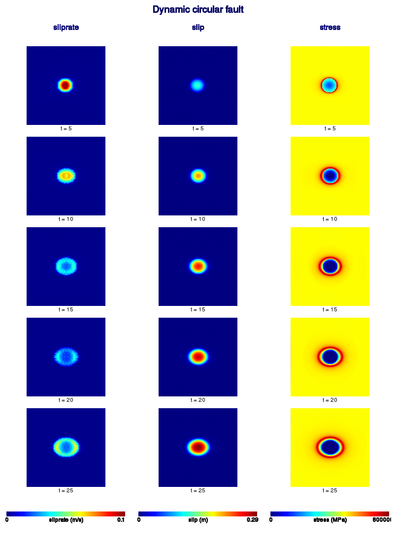
Figure 2. The plot_fault.gif file produced by the circular crack problem
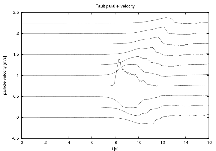
Figure 3. Velocity Seismograms along a perpendicular to the fault computed by fd3d_xy