GPS : HOW AND WHAT FOR ?
What is GPS ?
Since the end of the 70's, one of the main concerns of the american
"Department of Defense" (DoD), has been to concieve a system which will allow
any element of the american army (planes, ships, submarines, tanks, ground
troups) to know their position precisely and instantaneously, anytime and
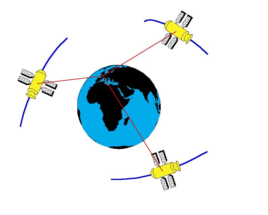
anywhere on the earth surface. The Global Positioning System (GPS) was built to
fulfill this task.
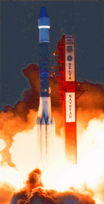
|

Launch of a GPS satellite
|

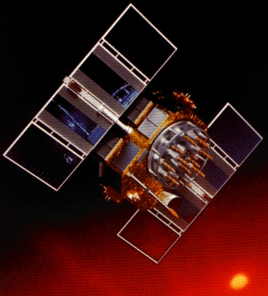
a GPS satellite
|
Commercial applications
Scientific applications
The precision achieved by pseudo-range measurements is not good enough
for most of the GPS applications in geophysics. For plate tectonic for exemple,
it is required that measurements be precise at the centimeter level (even
millimeter), if one is to be able to detect motions of a few centimeters per
year (or less) without having to wait
Again, to prevent potential "hostiles" to be able to get precise positions from
GPS, the system was built with the capacity to degrade its precison. This is
achieved by artificial degradation of the precision with which a certain number
of parameters are broadcasted by the satellites. For any of those numbers, the
last "byte" which contains the final digits (and therefore the full precision)
is deliberately jammed, that is single bit positions are exchanged using an
unknown algorithm. This dithering, known as Selective Availability, affects
first the clock of the satellites which gives the time tag for signal emission,
and second the satellite orbits which give the position of the emission point.
In practical, it is possible to go around this problem by using differential
GPS. This technique consists in using a reference station which position is
known with accurate precision. At every momment, the difference between the
wrong measured position and the true known position is radio broadcasted as a
correction valid in the whole area of the reference station.
for hundred of years to generate sizeable displacements. Then, a different
technique is applied. It consists in acquiring measurements of the
satellite-station distance directely on the carrier wave of the GPS signal
(phase measurements). In principal it is similar to pseudo-range measurements,
except that the wavelength (or characteristic size) of the signal is
considerabely reduced, which allows a far better precision.
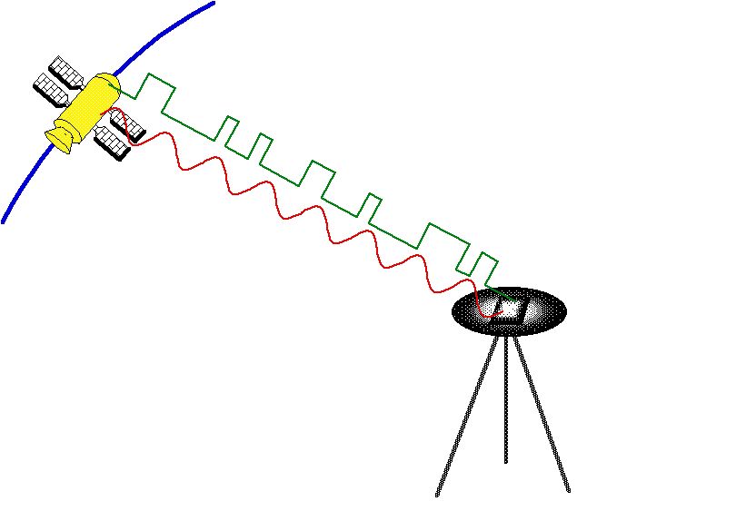
|

GPS signal ambiguity
|
For a complete mathematical theoryof GPS measurements processing (following R.W. King et al., 1985).....
Phenomenon affecting phase measurements precision
In addition to volunteer degradation of the signal quality by the
american military, there are number of natural causes which limit the precision
of the GPS positioning. Among them and by order of importance : Ionospheric and
Tropospheric refraction, GPS satellite orbits precision, multipath effects, and
position of the phase center of the GPS antennas. Some of these effects can be
accounted for in a more or less satisfying way, others are almost out of
control.
Ionospheric refraction
The Ionosphere, as stated by its name, is an enveloppe around the Earth
made of electrical particules (ions) which orbit at an altitude higher than 20
km. The carrier wave of the GPS signal has to travel through this layer on its
way from the satellite to the station. The simple fact that this layer is non
neutral implies a perturbation of the velocity of any electromagnetic wave going
through it. The amplitude of this perturbation is related to the wavelength and
to the density of electric particules in the medium, which density is unknown
and changes in space and with time. Terefore, the travel time of the GPS wave
will be affected by an unknown quantity, named ionospheric delay, and finally
the inferred distance between the satellite and the station will be wrong.
The solution consists in emitting two different waves on two different
frequencies. Each of them will be affected by a different amount, and the
comparison will give an evaluation of the ionospheric delay for all wavelengths.
It is for this very reason that the GPS system is "dual-frequency", which means
that two slightely different waves are emitted (1.575 GHz and 1.228 Ghz).
Nevertheless, whenever the Ionosphere is not in a steady state, in case of a
solar storm for exemple, the evaluation of the ionospheric delay remains
approximative and the precision of the measurement questionnable.
Tropospheric refraction
In the same way, the travel time of the GPS wave is affected by the
water vapor contains of the lower atmospheric layer (from 0 to 10 km altitude) :
the Troposphere. Therefore, it would be necessary to
know this quantity with precision along all the travel path followed by the
wave. This turns out to be an impossible task, even with the dual frequency
system. Since the perturbation introduced is more complicated than a simple time
ratio related to water vapor percentage, the differenciation between the two
waves does not produce the requested information : the tropospheric delay. There
are different techniques to adress this problem, neither of which being fully
satisfactory. The simplest one consists in simply putting an additional unknown
in the computations : the tropospheric delay itself. Nevertheless, since this
parameter changes along with meteorological conditions, it is necessary to
modify its value as time passes (every two hours for exemple). Eventually, this
leads to the introduction of many unknowns, which makes the computations less
stable and the results more questionnable.
In practical this problem is important when meteorological conditions
and tropospheric layer thickness are different from one location to another. The
baseline between two stations, one being located near the sea (at zero
altitude) with a high hygrometric level and the other one in high mountain
ranges with dry air, will be mostly affected. Finally, this error will show up
mostly on the vertical component of the baseline (the stations altitude
difference). The horizontal components will be less affected because the errors
will more or less average out since the satellites cover all azimuthal
directions (when the elevation coverage is restricted to the above horizon
satellites). From the theoretical point of view, instruments which allow to
directely measure the water vapor containts along the GPS wave path are
currently under experimentation. Yet, it is to soon to tell if such
measurements, based on sky brillance temperature, can be made accurate enough
for precise GPS applications.
GPS satellite orbits precision
Clearly, if an error is made on the satellite position, this error will
directly map into the station position since it is inferred from the satellite
to station distance. Again, the baseline between two stations will be les
affected than the station positions. If the two stations are not too far away,
the satellite position error (indentical for the two stations) will cancel out
when differenciating. Nevertheless, the rule of thumb is that the relative error
on the orbit equals the relative error on the baseline. GPS satellite orbits
can be computed very accurately but they are broadcasted by the american
military with a lousy precision of only 200 m. Over an average altitude of
around 20,000 km, this leads to a proportional error of 10-5 (10 ppm), which is
an error of 10 cm on a 10 km baseline ! Such a large error is totaly
unacceptable for precise GPS positioning. Therefore, it absolutely necessary to
recompute GPS satellite orbits with precise orbitographic softwares. This is
done by using GPS data acquired at fiducial stations scatered on the earth
surface and maintained for this purpose by the International GPS Service (IGS),
on behalf of the international scientific comunity. Those recomputed orbits are
precise at 20 cm, or 10-9 (1 ppb), which leads to an error reduced to 1 mm on a
1000 km long baseline.
Multipaths
Those phenomenoms are among the most difficult to seize. It is very easy
to see that any reflecting object disposed close to the GPS antenna may reflect
part of the signal coming from the satellite towards this antenna. Acting
exactely as a mirror creating one's image when one looks at it, the reflecting
object will create an image of the GPS antenna. It is then the position of this
fake antenna which is measured instead of the one of the true antenna. Moreover,
as the satellite is moving on its orbit, the reflection angle on the "mirror"
changes, and the antenna image moves. Then, it is the positon of a moving fake
antenna which is being measured ! It is extremely difficult to analyse
theoretically the impact of such and such potentially reflecting object. It is
possible to shield the antenna against such parasite reflections, but the shield
has to be uncomplete since the direct signal has to reach the antenna. The only
solution is to avoid as much as possible multipath effects by eliminating all
potentially reflecting objects from the neighbourhood of the antenna, which is
not so easy when one realizes that the ground itself is such a reflector !
The position of the GPS antenna phase centers
When measuring the position of a GPS antenna, what is it that we
actually measure ? Actually, the hart of a GPS antenna is basically made of an
electric wires coal inside which the electromagnetic wave signal is converted
into an electric current. It is the position of the very point where the
conversion occurs (named antenna phase center) which is measured. But such a
point is not materially defined. It is a virtual point which position depends on
the angle of incidence of the wave with respect to the wire coal, that is with
the antenna itself. The phase center, and therefore the antenna measured
position can move several centimeters apart, depending on where the signal
comes from, that is where the satellites are ! Here again, the error will be
moreorless averaged out since GPS signals come from almost everywhere, thanks to
the good spatial coverage of the satellites. Nevertheless, and because
satellites cannot be recorded below our feet accross the Earth, a systematic
shift in the altitude is inevitable. It is possible to map the displacements of
an antenna phase center in the laboratory. Nevertheless, such measurements are
very difficult to make and corrections from them are to be used with caution. On
a practical point of view, the problem is solved by using only identical
antennas for a given survey and by orientating all of them towards the same
direction. This will make all antenna phase centers move in the same direction
at the same time, and then baselines will remain constant although the points at
their ends will change position. Here again were are conducted to doing
relative positioning instead of absolute positioning.
Plate tectonics measured by GPS
The Wegener hypothesis of continental drift was confirmed twenty years
ago and since then by numbers of geophysical observations. Among those, the most
striking is the discovery of magnetic strips, parallel to the ridge and
successively positive and negative, "printed" in the ocean floors. Ocean floors
are made of the lava flowing out of the ridge. As they cool down, the rocks trap
the current Earth magnetic field. Because inversions of the magnetic field
polarity occured many times in the past, successive negative and positive values
of the field are captured. Therefore, the "zebra skin" of the ocean floors
gives a strong evidence for oceanic expension and for plate tectonics. Velocity
of this continental drift were estimated from the age of these strips and their
size. Similarly, it is possible to estimate the shift in between two sides of a
given structure separated by a fault (an old volcano or a fossile river bed for
example). Again, the evaluation of the age of the event will give an estimation
of the speed along the fault.
The major drawback of these methods lies in the fact that they give an
estimation of the velocity averaged on the geological time scale. Instantaneous
velocities can be very different from their average on long time scales.
Therefore, it is essential that present day velocities can be measured
directely. Among all the existing tools of geodesy (ground theodolites and
distance meters, space devices like VLBI, SLR, LLR, DORIS), GPS is very well
suited to the measurement of the deformation in a given area. Thanks to it good
precision, to its relatively low cost, to its operating facility, and to the
fact that it does not require site inter-visibility, it is possible to make a
large number of measurements quickly and cheapely on the studied area.
The principle is quite simple. A geodetic point is materialized by a
reference mark, typically a metal pin dug in an outcrop solidely tied to the
bedrock. Using a tripod and an optical device it is possible to center the GPS
antenna exactely on top of the bench mark, at a determined hight. Therefore, the
position of the reference mark can be easely deduced from the measured position
of the GPS antenna. By remeasuring the position of the benchmark after a given
time span it is possible to detect a displacement and deduce a velocity. The
deformation in a given area will be deduced from the displacements of many
points measured in the area. These many points just make a geodetic network.
Practically, since we must do a large number of differential measurements to
achieve a good precision, it is necessary to measure all points simultaneously
during many hours and even several days. Typically, at all stations, one measure
will be recorded every 30 seconds on all available satellites at every momment
during 3 full days. This represents an average of 30,000 to 40,000 measures by
point. Of course, the total measurement time span is given by the required
precision of the survey : 3 days for sub-centimetric precision over large scale
networks, but only one hour for very short baselines (less than 1 km) or if
sub-decimetric precision is enough.
Other applications
GPS is a formidable tool for positioning, and the simple fact of being able to
measure the position of a given point with a very good accuracy opens the way to
a great number of scientific applications.
Surveying an active fault
Naturally, the american scientists were the first to envision the
application of GPS aibilities to geophysical applications. On the other hand,
one of the major concerns of the authorities in this field is to study the
seismic hazards in California. In this area of the world, the sliding of two
tectonic plates along the San Andreas fault induces many devastating earthquakes
like those of San Francisco and Los Angeles lately. By measuring the positions
of points regularly scattered on both sides of the fault, and by looking at the
motions of those points, it is possible to map the fault very accurately. The
analysis of ground deformation in the vincinity of the fault gives basic
informations on the fracture depth, the length of the active segments, and
allows to define areas where the seismic risk is the more important.
Moreover, immediately after an earthquake, the GPS measure gives access
to the total displacement of the ground generated by the quake. This information
is decisive for the study of the fondamental mechanisms which govern seismic
rupture. Lastly, it is even possible to measure the positions of GPS points
during an earthquake. By computing the point positions at every measurement, one
can literally see the points moving during the couple of minutes the quake
lasts. If those points are well placed, one can see the propagation of the
rupture along the fault. Here again those informations allow to analyse the
seismic waves propagation and the induced ground motions. This type of network,
dedicated to monitoring an active fault, are now being developped in different
areas around the world : Japan, Indonesia,
Myanmar, and Turkey for exemple.
Monitoring volcanos
In the same way, it is possible to observe the deformations of the cone
of an active volcano. With just a few GPS points adequately placed an measured
continuously, it is possible to follow day after day the deformations due to the
rise of the lava flow. These measurements are usefull to volcanologist to
quantify the phenomenons associated with an eruption. One can also envision to
acquire some predictive capabilities, once these phenomenons are well
understood. Presently, such GPS measurements are conducted on different volcanos
like "le Piton de la fournaise" and "la Souffričre" in the french Antilles, and
the Merapi in Java, Indonesia.
"Post glacial rebound" and its implications on global change
Since a couple of years, it has been suspected that the sea level is
constantly rising. Although the numbers may be very small, a couple of
millimeters per year at most, this is a major concern for the whole planet. It
is very difficult to confirm this hypothesis and to find the precise numbers
because sea level variations are mixed with continents uplift or subsidence.
Localy, those tectonic motions can very well induce a sea level decrease, even
though the ocean surface is globaly rising (if the shore is rising faster for
example). On the other hand, if the sea level is rising, the water must come
from somewhere. It was suggested that global warming of the planet would "melt"
the polar ice sheets, and therefore free an important amount of liquid water in
the oceans. Although it would take thousands of years of warming to start to
really melt the Antarctic ice sheet, a small change of the thermal conditions
can generate large variations in the speed of the glaciers. This could easely
affect the total amount of water released in the ocean. By liberating water,
such a phenomenon would generate a decrease of the mass of the ice sheet. An
uplift of the continent underneath would therefore take place as its load
decreases. Such an effect took place in the past in the Canadian Laurentides and
in northern Europe during and after the deglaciation periods. Using GPS, it is
possible to measure the possible uplift of the Antarctic continent induced by
the ice sheet mass decrease. A quantification of the uplift would allow a
quantification of the amount of water send in the oceans, and therefore assess
the risk of sea level rise. Such measurements (Antarctica)
started a couple of years ago and results are coming out presently.
Measuring of the geoid
Because of density anomalies inside the planet, the Earth gravity field
is not the one of an homogenous sphere flattened at the poles. On the opposite,
it shows swells and holes in accordance with the density of the rocks in the
crust and below, and the elevation of the topography. Where the Earth surface is
covered by oceans, the liquid water goes freely where the gravity is stronger,
to reach an equilibrium at an higher alitude until the gravity is equal along
the water surface. The ondulated surface thus generated is called the Geoid. Of
course the geoid exists also over the continents, although it is not
materialized by the presence of water.
The knowledge of the Geoid is of first importance to geophysicist.
Because it is affected by masses deep in the Earth mantle, the Geoid gives
precise indications on the density and composition of the deep interior of the
planet. Over the oceans, the Geoid is known from altimetric satellites which
simply measure the altitude of the sea level. Nevertheless, and because it is
not materialized over solid surfaces, the continental Geoid is difficult to
measure and remains not very well known. Now, the GPS system, because it uses
satellites which orbit around the Earth center of
mass, gives the position with respect to this reference system. That is to say
that one knows the distance between a GPS point and the Earth center. Then, it
is enough to know the altitude of this point (ie. its relative hight to the
ocean level) and the difference between the two is simply the Geoid !
Measuring of erosion
Last, it is possible to use the GPS system in a slightely different
manner. This application uses the navigation reasoning, but keeps the principle
of the phase measurements which allow accurate enough positioning. By making
measurements very frequently, it is possible to follow the trajectory of a
mobile receiver. Each measure gives the position (latitude, longitude, and
altitude) of the receiver as a function of time. Because their is only one
measure for each position, the latter is known with a degraded precision.
Nevertheless, the receiver position at a given time is related by its velocity
to its positions just before and immediately after. Finally, it is possible to
reconstruct the trajectory of the receiver with a sub decimetric precision.
Doing this, it is possible to make a precise topographic map (altitude versus
latitude and longitude) of a given area covered by a GPS receiver placed on a
car or on human back. This is very easy to do on the sea shore, where it is
possible to map the sand dunes and the inter tidal area uncovered by the sea at
low tide (Merlimont). It is even possible to map the topography of the sand banks below the
water level by coupling the GPS receiverto a depthmeter (SONAR). By
measuring these topographies at regular interval, or immediately after a storm, it is
possible to directely monitor the effects of slow and continuous erosion or
catastrophic events, as well as quantify the amount of material (sand) involved
and the paths it followed. These techniques are presently being tested on the
french northern sea shore.
Encarts
1-Pseudo-range codes and access policy of the DoD
Hence, there are two types of pseudo-distance which allow different precisions :
The C/A (Coarse Acquisition) code, available to all potential users,
which allows a precision of around 100 m. It is this signal which is recorded in
most commercial GPS receivers used for navigation purposes (ships, airplanes,
and parisien taxis)
The P (Precise) code, encrypted to deny access to anyone else but the
american army, which allows a precision of around 10 m. This P-code encryption
scheme, known as "Anti Spoofing", was designed to deny access to potential
ennemy at wartime but has been in fact activated permanently since the beginning
of 1994.
Again, to prevent potential "hostiles" to be able to get precise positions from GPS,
the system was built with the capacity to degrade its precision. This is achivied by
artificial degradation of the precision with which a certain number of parameters are
broadcasted by the satellites. For any of those numbers, the last "byte" which contains
the final digits (and therefore the full precision) is deliberately jammed, that is
single bits positions are exchanged using an unknown algorithm. This dithering, know
as Selective availability, affects first the clock of the satellites which gives the
time tag for signal emission, and second the satellite orbits which give the position
of the emission point. In practical, it is possible to go around this problem by using
differential GPS. This technique consists in using a reference station which position
is known with accurate position. At everey momment, the difference between the wrong
measured position and the true known poisition is radio broadcasted as a correction
valid in the whole area of the reference station.
2-Carrier beat phase measurements
The wavelength, or characteristic size of the signal, is reduced from 30 m for
C/A-code and 3 m for P-code to 19 cm for the carrier wave of the first one and
24 cm for the carrier of the second one. It is possible to measure a time shift
between to waves with an accuracy up to a fraction of one wavelength. Therefore,
measurements based on the carrier wave phase can achieve a sub centimetric
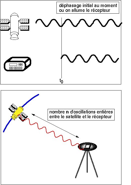
precision. Nevertheless, this technique has a major drawback : phase
measurements are fondamentaly ambiguous. When different (therefore
identificable) crenels follow each other in the pseudo-range signal, nothing
allows the identification of one wavelength from the previous or the following
one : they are all strictly identical. In other words, the actual number of
oscillations from the satellite to the station remains unknown. What is known is
the number of oscillations which separate two measurements made on the same
satellite at two different times. Therefore, there is no direct access to the
distance satellite-station and then no real time direct measure of the station
position. On the other hand, after continuous measurements have been recorded on
all available satellites for a given time, one disposes of a large number of
equations (as many as recorded measurements) for a small number of unknowns (3
for station position and 1 for each satellite-station distance at the first
measurement). The technique consists then in acquiring as many measurement as
possible, record them, and process the equations system with a computer while
back in the laboratory. Also, to eliminate the inauspicious effects of the
Selective Availability, it is necessary to combine data from different stations
(again differential GPS). This allows to cancel the errors from the satellite
clocks by paying the cost of loosing absolute positioning. Therefore, only
distances between stations are known and not station positions. In geodesy,
those distances are called baselines and have three components : one vertical
component which corresponds to the altitude difference between the stations, and
two horizontal components which are the distances between the stations along
the North-South and East-West directions.
3-Cost of GPS receivers
A commercial receiver used for navigation purposes will be able to measure only
the coarse pseudo range distances coded on one of the two frequencies. Such
receivers are available from 1500 FF or 300 USD. On the opposite, dual frequency
receivers able to measure both pseudo-range and phase data on both carrier
waves cost up to 150,000 FF or 30,000 USD. There is an intermediate category of
receivers which allow relatively precise positioning without being excessively
costly. Those are the single frequency receivers, which measure pseudo-range and
phase data on only one of the two wavelength. Acquiring data only on the
frequency with the higher signal/noise ratio, those receivers are built with
relatively cheap electronic.
 PostScript file
 Return to index